3. Implementing VAE with PyTorch
In part 1 and 2, we discussed variational inference and ELBO loss which converted the problem of modelling the data distribution into an optimization problem. We also discussed the EM algorithm and the mini batch stochastic gradient descent algorithm to solve the optimization problem.
With this information, let’s implement the original Variational Auto Encoder model with the PyTorch library for our problem of generating images. In this part, we will use the Flowers102 dataset to learn a probability distribution over 32x32x3 = 3072 dimensional space. The learnt distribution should assign high probabilities to 3072 dimensional vectors that look like flowers (when represented as 32x32 RGB images) similar to ones in the dataset.
Directory Structure
Throughout this series, we will follow some guidelines on structuring our code. To begin with, we will have a directory structure as follows
root
    experiments.ipynb
    vae_training.py
    gan_training.py
    ...
    datasets
        dtd
        preprocessing.py
    vae
        layers.py
        losses.py
        vae.py
    gan
        layers.py
        losses.py
        gan.py
    ...
The root directory will hold all the code used in this series.
It will contain one folder for all datasets. Each dataset will have their own folder within it. Each model type will have a separate folder for it. The data preprocessing logic, building block layers, loss functions will reside in their own files for every model type. The file with the same name as the folder will hold the final models constructor.
Each model type will have its own training and inference script in the root folder. We will also have some Jupyter notebooks, like experiments.ipynb, to play around and try out individual pieces of code.
As much as possible, we will follow the guidelines posted in this unofficial PyTorch style guide.
Data
We will use the Flowers102 dataset containing images of 102 types of flowers, each type having from 40 to 258 images. Our task will be to capture different attributes of flowers in a small $N$ dimensional latent space ($N$ could be as small as 10) and generate new unique flower images similar to a provided image.
Flowers102 is available for use with the torchvision datasets API and the official documents has a good tutorial on using it.
Model
We will divide the model into 3 modular blocks -
- Encoder - This block accepts a batch of images and outputs a batch of multidimensional means and standard deviations. Therefore the input shape is
[batch, image_channels, image_width, image_height]and output consists of 2 tensors, each of shape[batch, latent_dimension]. Technically, the standard deviations should be of shape[batch, latent_dimension, latent_dimension]but since we assume the output distribution is a mixture of Gaussians with diagonal covariance, we only output values on the diagonal. The value ofimage_channelsis 3 for RGB images. - SampleLatent - This block accepts a batch of multidimensional means and standard deviations and outputs a batch of latent vectors sampled from multivariate Gaussian of those means and a covariance matrix constructed from those diagonal standard deviations. Therefore the input accepts 2 tensors of shape
[batch, latent_dimension]and output is a tensor of shape[batch, latent_dimension]. This block will use the re-parametrisation trick to enable computation of gradients of loss w.r.t parameters of encoder. - Decoder - This block accepts a batch of latent vectors and outputs a batch of 3 channelled (RGB) images. Note that this block does not output means and covariances of the multivariate Gaussian that governs the data. We assume that the decoder output distribution has constant covariance matrix. Then, when we will minimise the negative log probability of the original image w.r.t this Gaussian, we will end up minimising the a value proportional to mean squared error between the mean image output by the decoder and the original image i.e. the reconstruction error. You could also output and use a covariance matrix. Since our images are high dimensional, this would end up being a huge matrix though. The assumption helps us simplify the computation. So, the decoder accepts
[batch, latent_dimension]as input and outputs[batch, 3, image_width, image_height]as mean of the output Gaussian given the latent. The mean of a multivariate Gaussian should technically be a 1D vector of size3 * image_width * image_heightbut this is just a reshaped version of it.
Training loop
The main training loop is defined in the vae_training.py file.
import torch
from torch.utils.data import DataLoader
from torch.utils.tensorboard import SummaryWriter
from vae.vae import VAE
from vae.losses import ELBOLoss
from torchvision import datasets
from torchvision.transforms import ToTensor, Resize, Compose
from torchvision.utils import save_image, make_grid

LOG_DIR = "./generative_modelling/vae/runs"
DATASET_ROOT = "./generative_modelling/datasets"

# Instantiate a TensorBoard SummaryWriter to log data and view on TensorBoard
writer = SummaryWriter(LOG_DIR)

# We will operate on 32x32 resolution images
# Therefore, we create a data transformation pipeline that takes every image
# and resizes it to 32x32 resolution and converts it to a PyTorch tensor
dataset_transformation_pipeline = Compose([Resize((32, 32)), ToTensor()])

# Load training and test datasets using the data transformation pipeline
training_data = datasets.Flowers102(root=f"{DATASET_ROOT}/train/", download=True, split="train", transform=dataset_transformation_pipeline)
test_data = datasets.Flowers102(root=f"{DATASET_ROOT}/test/", download=True, split="test", transform=dataset_transformation_pipeline)

# Use the datasets to create dataloaders that will shuffle and batch data
train_dataloader = DataLoader(training_data, batch_size=64, shuffle=True)
test_dataloader = DataLoader(test_data, batch_size=5, shuffle=True)
# For test dataset, create an iterator so that
# we can call next() on it at end of every epoch
test_dataiterator = iter(test_dataloader)

# Initialize model, loss and optimiser
num_epochs = 500
model = VAE(image_resolution=(32, 32), image_channels=3, latent_size=10)
loss = ELBOLoss(beta=0.1)
optimiser = torch.optim.Adam(model.parameters(), lr=0.0001)

# Main training loop
batch_num = 0
for epoch in range(num_epochs):
    for i, (train_features, train_labels) in enumerate(train_dataloader):
        # Step 1: zero gradients of optimizer
        optimiser.zero_grad()
        # Step 2: forward pass through the model
        reconstructions, means, log_vars = model(train_features)
        # Step 3: calculate loss
        beta, kl_loss, reconstruction_loss, total_loss = loss(train_features, reconstructions, means, log_vars)
        # Step 4: write loss to tensorboard
        writer.add_scalars("loss", {"KL Loss": kl_loss, "Reconstruction Loss": reconstruction_loss, "Total Loss": total_loss}, batch_num)
        # Step 5: compute gradients
        total_loss.backward()
        # Step 6: apply gradient descent step
        optimiser.step()
        batch_num += 1

    # At end of every epoch, create reconstructions on one batch of test data
    (test_features, _) = next(test_dataiterator)
    reconstructions, means, log_vars = model(test_features)
    grid = make_grid(test_features)
    writer.add_image('originals', grid, epoch)
    grid = make_grid(reconstructions)
    writer.add_image('reconstructions', grid, epoch)

    print(f"Epoch: {epoch}, Reconstruction Loss: {reconstruction_loss:.2f}, KL Loss: {kl_loss:.2f}, Total Loss: {total_loss:.2f}")
Model
The VAE model is defined in vae/vae.py. The model file is kept simple while hiding details of encoder, decoder and sampling using reparametrization trick in vae.layers.
from torch import nn
from vae.layers import Decoder, Encoder, SampleLatent

class VAE(nn.Module):
    def __init__(self, image_resolution: int, latent_size: int, image_channels):
        super(VAE, self).__init__()
        self.encoder = Encoder(image_resolution, image_channels, latent_size)
        self.sample_latent = SampleLatent(latent_size)
        self.decoder = Decoder(image_resolution, image_channels, latent_size)

    def forward(self, x):
        # x is batch of images of shape [batch_size, height, width, channels]
        mean, log_var = self.encoder(x)
        # Encoder generates a [batch_size, latent_size] shaped mean
        # and [batch_size, latent_size] shaped log of variance
        latent_sample = self.sample_latent(mean, log_var)
        # latent_sample has shape [batch_size, latent_size]
        # sampled from an isotropic multivariate Gaussian distribution
        # described by mean and log_var
        reconstruction = self.decoder(latent_sample)
        # decoder reconstructs [batch_size, height, width, channels]
        # from batch_size samples from latent space
        return reconstruction, mean, log_var
Layers
The encoder, decoder and sampling layers are defined in vae/layers.py.
import torch
from torch import nn

class SampleLatent(nn.Module):
    def __init__(self, latent_size: int):
        super(SampleLatent, self).__init__()
        self.latent_size = latent_size

    def forward(self, mean, log_var):
        batch_size = mean.shape[0]
        epsilon = torch.normal(0.0, 1.0, (batch_size, self.latent_size))
        return torch.exp(0.5 * log_var) * epsilon + mean

class Encoder(nn.Module):
    def __init__(self, image_resolution, image_channels, latent_size):
        super().__init__()
        (w, h) = image_resolution
        self.conv1 = nn.Conv2d(in_channels=image_channels, out_channels=16, kernel_size=3, stride=1, padding="same")
        self.act1 = nn.ReLU()
        self.pool1 = nn.MaxPool2d(kernel_size=2)
        self.conv2 = nn.Conv2d(in_channels=16, out_channels=32, kernel_size=3, stride=1, padding="same")
        self.act2 = nn.ReLU()
        self.pool2 = nn.MaxPool2d(kernel_size=2)
        self.conv3 = nn.Conv2d(in_channels=32, out_channels=64, kernel_size=3, stride=1, padding="same")
        self.act3 = nn.ReLU()
        self.pool3 = nn.MaxPool2d(kernel_size=2)
        self.flatten = nn.Flatten()
        self.fcm = nn.Linear(64 * (w // 8) * (h // 8), 10)
        self.fcv = nn.Linear(64 * (w // 8) * (h // 8), 10)

    def forward(self, x):
        x = self.conv1(x)
        x = self.act1(x)
        x = self.pool1(x)
        x = self.conv2(x)
        x = self.act2(x)
        x = self.pool2(x)
        x = self.conv3(x)
        x = self.act3(x)
        x = self.pool3(x)
        x = self.flatten(x)
        return self.fcm(x), self.fcv(x)

class Decoder(nn.Module):
    def __init__(self, image_resolution, image_channels, latent_size):
        super().__init__()
        (self.w , self.h) = image_resolution
        self.fc = nn.Linear(10, 64 * (self.w // 8) * (self.h // 8))
        self.deconv1 = nn.ConvTranspose2d(in_channels=64, out_channels=32, kernel_size=2, stride=2)
        self.act1 = nn.ReLU()
        self.deconv2 = nn.ConvTranspose2d(in_channels=32, out_channels=16, kernel_size=2, stride=2)
        self.act2 = nn.ReLU()
        self.deconv3 = nn.ConvTranspose2d(in_channels=16, out_channels=image_channels, kernel_size=2, stride=2)
        self.act3 = nn.Sigmoid()

    def forward(self, x):
        x = self.fc(x)
        x = x.reshape((-1, 64, (self.w // 8), (self.h // 8)))
        x = self.deconv1(x)
        x = self.act1(x)
        x = self.deconv2(x)
        x = self.act2(x)
        x = self.deconv3(x)
        return self.act3(x)
Loss
The ELBO loss function is defined in vae/loss.py. In practice, weighing the KL loss and the reconstruction loss differently helps SGD converge better. Therefore, we use a parameter beta to weigh KL loss term relative to the reconstruction loss term.
from torch import nn
import torch

class ELBOLoss(nn.Module):
    def __init__(self, beta):
        super(ELBOLoss, self).__init__()
        self.beta = beta

    def forward(self, original, reconstruction, latent_mean, latent_log_var):
        kl_loss = self.kl_loss(latent_mean, latent_log_var)
        reconstruction_loss = self.reconstruction_loss(original, reconstruction)
        total_loss = self.beta*kl_loss + reconstruction_loss
        return self.beta, kl_loss, reconstruction_loss, total_loss

    def kl_loss(self, latent_mean, latent_log_var):
        kl_loss = -0.5 * torch.sum( 1 + latent_log_var - torch.square(latent_mean) - torch.exp(latent_log_var), -1 )
        return torch.mean(kl_loss)

    def reconstruction_loss(self, original, reconstruction):
        return torch.mean(torch.sum(torch.square(original - reconstruction), dim=(1,2,3)))
Practical Aspects of VAE
In practice, the entire domain of deep learning is about aiding stochastic mini batch gradient descent (SGD) to solve our optimization problem. In order to do this, we will introduce some “hacks”. These are modifications to the objective function or training procedure in order to either reduce/parallelize computation or to aide stochastic mini batch gradient descent. In the previous post, we have seen one such hack that the original VAE paper used where we sample just 1 latent vector to get a Monte Carlo estimate for ELBO.
We will introduce a few more modifications that will help train the VAE with SGD. They are summarized here -
Modifications to reduce computation
- We will reduce the image size. For the purposes of this series, we will use images of dimension 64x64 pixels. This is just enough resolution to capture our patterns.
- We will modify the conditional distribution $P(x | z, \theta)$ as one of the two -
- A 4,096 (64 x 64) dimensional Gaussian with constant diagonal covariance matrix. With this, the output of our decoder function is just the mean of the Gaussian. Since covariance is constant, minimizing $\log P(x_i|z_i,\theta)$, is equivalent to minimizing the mean squared error between the pixels in output of our decoder (the mean) and the input image that led to the latent vector and the reconstruction mean. This transforms the first part of our ELBO loss into a mean squared error between matrices with 4,096 entries.
- A joint distribution of 4.096 independent Bernoulli distributions, that is, each pixel in the image has a Bernoulli distribution that is independent of other pixels. For this, the values of input image are normalized to fall between 0 and 1. Each element of output of decoder is also restricted to be between 0 and 1 (using a Sigmoid activation). This transforms the first part of our ELBO loss to sum of binary cross entropy between each pixel of the two images.
Modifications to aide SGD
- If we train the VAE with the ELBO loss, we will observe the the second part of ELBO, i.e. the KL divergence between posterior and prior goes to 0 much faster than the reconstruction error. Once that happens, the latent vector is always sampled from a standard normal Gaussian and the reconstructions will all look similar brown and heavily blurred images. To counter that, we introduce a training scheme that places very low weight on the KL divergence part of ELBO loss during initial stages of training. Experimental research has suggested a few different types of schemes for varying the weights of the two parts of the ELBO loss.
- We will use Batch Normalization layers whose dynamics have not been part of the derivations we have discussed till now. The original paper which introduced batch normalization does a great job of explaining how it aides SGD.
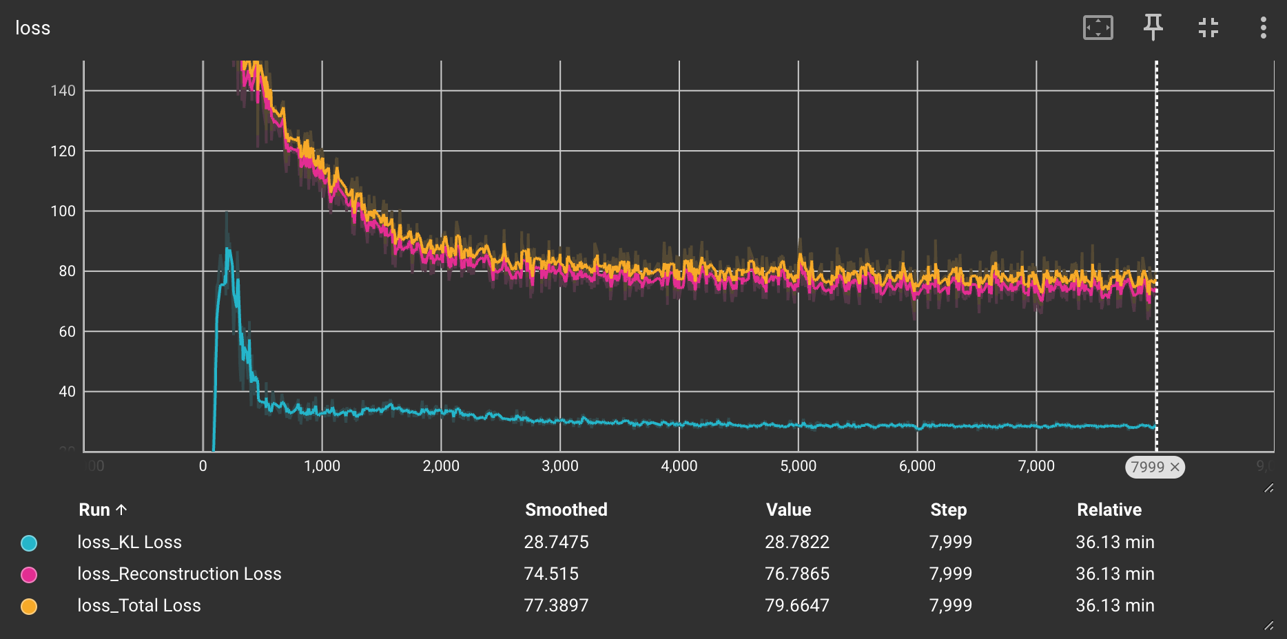
Results
The following chart shows the tensorboard graph of loss components.
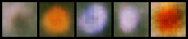
After around 30 epochs, the decoder has started learning average location of flower colors as response to minimizing average reconstruction error
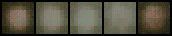
By 200th epoch, the decoder has started generating images that show hints of being flowers
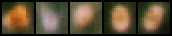
By 350th epoch, we start seeing blurry reconstructions of flowers (odd rows are original, even rows are their reconstructions),